Where Do Variable Coefficient Problems Come From?
Overview
We have now learned the basics of solving linear differential equations with polynomial coefficients. Usually at the end of a unit we spend a couple of days on an application or two to show how such problems arise and how the techniques we've learned can be applied. Unfortunately, the problems that give rise to equations of the form studied in chapter 4 are usually quite complicated. It is very rare to encounter a circuit where the resistance is given by some polynomial (though Edgar Allan Poe did write a memorable story about a pendulum whose length grew with time). In this section I will touch on two examples of situations where the analysis leads to differential equations with variable coefficients.Partial Differential Equations
The first and perhaps most common situation is when we start with a problem in higher dimensions, which we solve by reducing it to several problems in one dimension. A constant coefficient higher dimensional problem can create a variable coefficient problem in one dimension depending on the geometry. As an example where 2-dimensional geometry can lead to polynomial coefficients in one dimension, consider Laplace's equation in two dimensions $$ \frac{\partial^2u}{\partial x^2} + \frac{\partial^2u}{\partial y^2} = 0 $$ where our region is the unit disk. This equation arises in the study of electric potential and of steady-state temperature. For example, suppose I have a uniform disk and I know the temperature at each point along its (circular) boundary. Suppose the disk is insulated and has been left to reach a steady-state temperature. Then $\displaystyle \frac{\partial^2u}{\partial x^2} + \frac{\partial^2u}{\partial y^2} = 0$ where $u$ is the temperature at the point $(x,y)$. Now we also need to write down the boundary conditions (which represent our knowledge of the temperature at the boundary). However, since the boundary is a circle, this can get a bit sticky if we insist on working in rectangular coordinates. Things will go smoother if we change to polar coordinates $$ \begin{align} r&=\sqrt{x^2+y^2} \\ \theta&=\arctan(y/x) \end{align} $$ The trouble comes when we need to use the chain rule for functions of several variables to convert $\displaystyle \frac{\partial^2u}{\partial x^2}$ and $\displaystyle \frac{\partial^2u}{\partial y^2}$ to polar coordinates. The process begins with $$ \begin{align} \frac{\partial u}{\partial x} &= \frac{\partial r}{\partial x}\frac{\partial u}{\partial r} + \frac{\partial \theta}{\partial x}\frac{\partial u}{\partial \theta} \\ &=\frac{x}{\sqrt{x^2+y^2}}\frac{\partial u}{\partial r} + \frac{-y}{x^2+y^2}\frac{\partial u}{\partial \theta} \\ &= \frac{r\cos(\theta)}{r}\frac{\partial u}{\partial r} - \frac{r\sin(\theta)}{r^2}\frac{\partial u}{\partial \theta} \\ &= \cos(\theta)\frac{\partial u}{\partial r} - \frac{\sin(\theta)}{r}\frac{\partial u}{\partial \theta} \end{align} $$ Then to get the second derivative we compute $$ \begin{align} \frac{\partial^2 u}{\partial x^2} = \frac{\partial}{\partial x}\left(\frac{\partial u}{\partial x}\right) &= \frac{\partial r}{\partial x}\left(\frac{\partial}{\partial r} \left(\frac{\partial u}{\partial x}\right)\right) +\frac{\partial \theta}{\partial x}\left(\frac{\partial}{\partial \theta} \left(\frac{\partial u}{\partial x}\right)\right) \\ &=\frac{\partial r}{\partial x} \left(\frac{\partial}{\partial r} \left(\cos(\theta)\frac{\partial u}{\partial r} - \frac{\sin(\theta)}{r}\frac{\partial u}{\partial \theta}\right)\right) + \frac{\partial \theta}{\partial x}\left( \frac{\partial}{\partial \theta}\left( \cos(\theta)\frac{\partial u}{\partial r} - \frac{\sin(\theta)}{r}\frac{\partial u}{\partial \theta} \right)\right) \\ &=\frac{x}{\sqrt{x^2+y^2}}\left(cos(\theta)\frac{\partial^2 u}{\partial r^2}-\left(\frac{\partial \sin(\theta)/r}{\partial r}\frac{\partial u}{\partial \theta} + \frac{\sin(\theta)}{r}\frac{\partial^2 u}{\partial r\partial\theta}\right)\right) \\ &\qquad\qquad + \frac{-y}{x^2+y^2}\left(\left(\frac{\partial \cos(\theta)}{\partial \theta}\frac{\partial u}{\partial r}+\cos(\theta)\frac{\partial^2 u}{\partial r\partial \theta}\right) - \left(\frac{\partial \sin(\theta)/r}{\partial \theta}\frac{\partial u}{\partial \theta} + \frac{\sin(\theta)}{r}\frac{\partial^2 u}{\partial\theta^2}\right)\right) \\ &=\cos(\theta)\left(\cos(\theta)\frac{\partial^2 u}{\partial r^2} +\frac{\sin(\theta)}{r^2}\frac{\partial u}{\partial \theta} - \frac{\sin(\theta)}{r}\frac{\partial^2 u}{\partial r\partial\theta} \right) \\ &\qquad\qquad - \frac{\sin(\theta)}{r}\left( -\sin(\theta)\frac{\partial u}{\partial r}+ \cos(\theta)\frac{\partial^2 u}{\partial r\partial \theta} -\frac{\cos(\theta)}{r}\frac{\partial u}{\partial \theta} - \frac{\sin(\theta)}{r}\frac{\partial^2 u}{\partial \theta^2} \right) \\ &=\cos^2(\theta)\frac{\partial^2 u}{\partial r^2} + 2\frac{\sin(\theta)\cos(\theta)}{r^2}\frac{\partial u}{\partial \theta} -2\frac{\sin(\theta)\cos(\theta)}{r}\frac{\partial^2 u}{\partial r\partial \theta} +\frac{\sin^2(\theta)}{r}\frac{\partial u}{\partial r} +\frac{\sin^2(\theta)}{r^2}\frac{\partial^2 u}{\partial \theta^2}. \end{align} $$ A similar calculation shows $$ \frac{\partial^2 u}{\partial y^2}= \sin^2(\theta)\frac{\partial^2 u}{\partial r^2} -2\frac{\sin(\theta)\cos(\theta)}{r^2}\frac{\partial u}{\partial \theta} +2\frac{\sin(\theta)\cos(\theta)}{r}\frac{\partial^2 u}{\partial r\partial \theta} + \frac{\cos^2(\theta)}{r}\frac{\partial u}{\partial r} +\frac{\cos^2(\theta)}{r^2}\frac{\partial^2 u}{\partial \theta^2} $$ Adding these up gives us $$ \frac{\partial^2 u}{\partial x^2}+\frac{\partial^2 u}{\partial y^2} = \frac{\partial^2 u}{\partial r^2} + \frac{1}{r}\frac{\partial u}{\partial r} + \frac{1}{r^2}\frac{\partial u}{\partial \theta^2} $$ So our equation for Laplace's equation with a known temperature on an insulated circular disk with radius 1 is the boundary value problem $$ \begin{align} \frac{\partial^2 u}{\partial r^2} + \frac{1}{r}\frac{\partial u}{\partial r} + \frac{1}{r^2}\frac{\partial u}{\partial \theta^2} &= 0 \\ u(1,\theta)&=f(\theta) \\ \frac{\partial u}{\partial r}(1,\theta)&=0 \end{align} $$ where $u(r,\theta)$ is the temperature function (in polar coordinates) and $r=1$ corresponds to the boundary of the disk, $f(\theta)$ is the function that represents the known temperature at the boundary, and $\displaystyle\frac{\partial u}{\partial r}$ is 0 at the boundary $r=1$ because the disk is insulated. Notice that our problem which began as constant coefficient has become variable coefficient when we changed from rectangular to polar coordinates. Now this is a partial differential equation. The basic trick that works here is to use "separation of variables" to split the problem from one partial differential equation in two coordinates to two ordinary differential equations, one in $r$ and one in $\theta$. You can go through the full details of this process in Math 632, Partial Differential Equations. But for us, this is an example of where a variable coefficient equation can arise in practice. There are also situations where you can reduce a first-order non-linear equation to a second-order linear, but not constant coefficient, equation. But I think the most interesting example of where variable coefficient problems arise that we haven't covered yet is when you start with the solution and then build the differential equation. In the section on Series Solutions, we solved Chebyshev's equation, $(1-x^2)y''-xy'+\alpha^2 y=0,$ and noted that, for every integer value for $\alpha,$ this equation has a solution which is a polynomial of degree $\alpha,$ called the Chebyshev polynomial. In this case the polynomials were actually developed first and the differential equation developed later in studying the polynomials.Chebyshev Polynomials
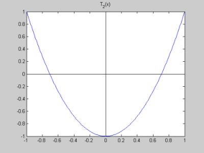
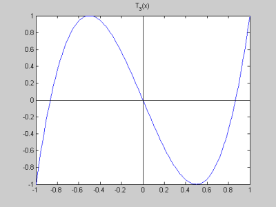
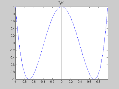
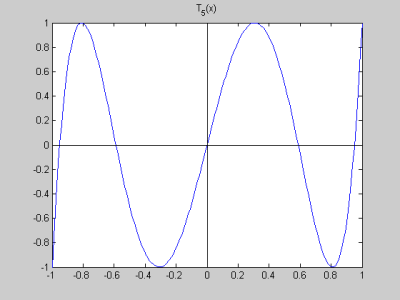
The Chebyshev polynomials are usually defined by the formula $T_n(x)=\cos(n\arccos(x))$ for $|x|\le 1$. Typically the first exercise is to show that these are polynomials; they look like trig functions at first glance. But some work with trig identities will show that the $T_n$ are actually polynomials. For example: $$ \begin{align} T_2(x)&=\cos(2\arccos(x)) \\ &=\cos^2(\arccos(x)) - \sin^2(\arccos(x)) \\ &=\cos^2(\arccos(x)) - (1 - \cos^2(\arccos(x))) \\ &= x^2 - (1-x^2) \\ &= 2x^2 -1 \end{align} $$ An important property of the $T_n(x)$ is that $-1 \le T_n(x) \le 1$ for all $-1 \le x \le 1.$ This follows immediately from the definition in terms of $\cos$ of course. In fact, the graphs of the $T_n(x)$ all have the equiripple property. That means they oscillate between -1 and 1 with each oscillation going the full distance to -1 and 1. See the graphs of several Chebyshev polynomials below. |
 |
 |
 |
If you have any problems with this page, please contact bennett@ksu.edu.
©1994-2025 Andrew G. Bennett