Kansas State University

Launch Systems App.

The solution of a system is a pair of functions, x(t) and y(t) (or even three or more functions depending on the size of the system). To view the solution, it is usually most helpful to consider (x(t), y(t)) as a parametric curve which can be plotted on the xy-plane. In this lab we will look at a variety of such curves and develop some ideas about how the pictures relate to the initial equation.

Launch the systems app. You can enter a constant-coefficient first-order system for x and y, along with a pair of initial values in the applet at the top of the page. If you press the "Update Graph" button it will draw the solution to the system as a parametric curve in blue. It will also draw two lines. The red line marks where x' = 0 and the green line marks where y' = 0. The arrows show the direction the blue parametric curve will travel when it crosses the line (as t increases). If you change the initial conditions without changing the equations, a new curve will be added to the current graph, with the old blue curve changing to gray so you can clearly distinguish the new curve from the old. The "Clear Old Curves" button will erase all the blue and gray curves if things get too confusing. If you change the equations, all the old curves will be automatically erased when you "Update Graph" as part of graphing the new system.

Questions

1. Experiment with different systems and initial values. Note that the solution curves are always horizontal when they cross the green line and vertical when they cross the red line. Why do the curves behave like that?

2. Now find examples of systems of each of the following 6 types of systems. Note that you don't have to find examples that look exactly like the pictures, just examples that that have the same sort of behavior. Of course, using the red and green lines you can actually match the pictures without much effort, and that is probably the easiest way to find examples of some of the behaviors.

   (A)	Solutions diverge straight out to infinity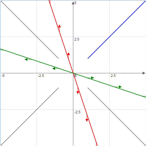
   (B)	Solutions converge directly to the origin (possibly with a "twist" as illustrated here).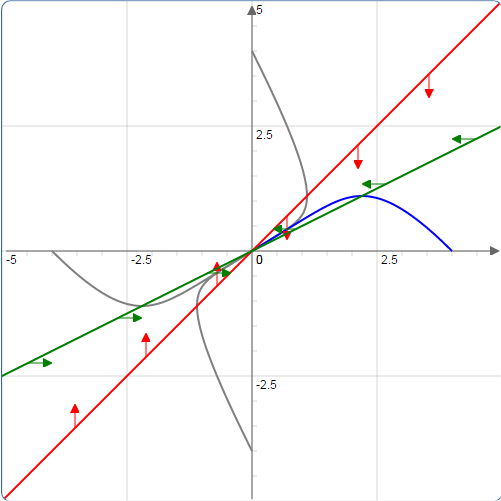
   (C)	A "saddle point" at (0,0) where solutions converge toward the origin in one direction and then turn and diverge away in a different direction (there will be one solution converging to the origin in between the solutions turning in each direction).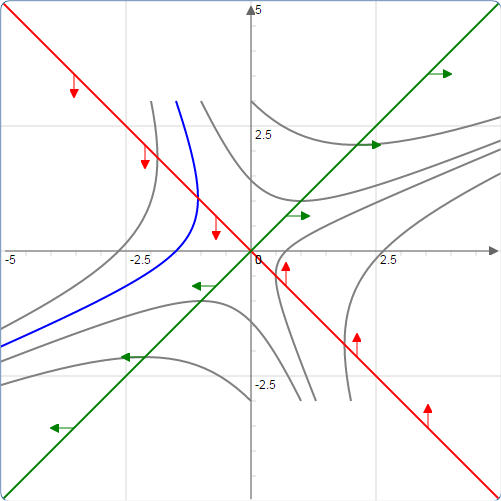
   (D)	Solutions spiral out to infinity.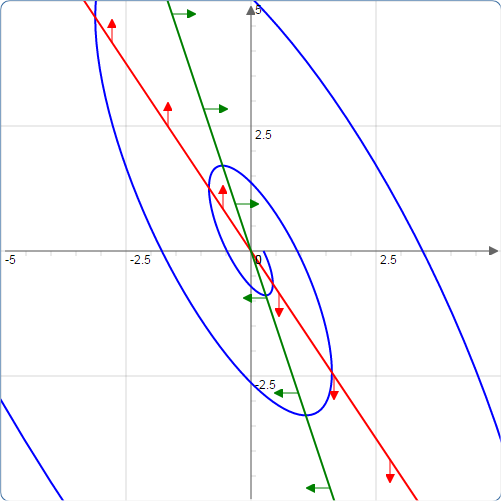
   (E)	Solutions spiral in to the origin.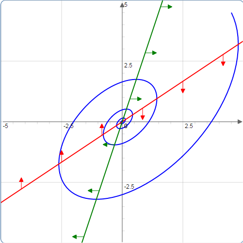
   (F)	Solutions spin around the origin along ellipses, neither converging toward the origin nor diverging away from it.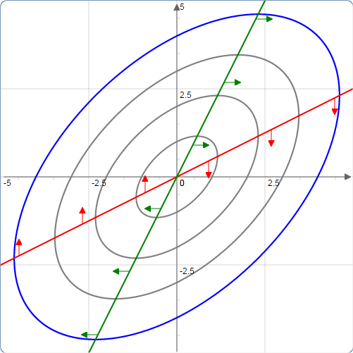

   ---

3. In the system
   x' = ax + by, x(0)=x₀,
   y' = cx + dy, y(0)=y₀,
   

   two very useful quantities to know are the trace = a + d and the determinant = ad - bc. Compute the trace and determinant for each of your examples. Can you find a relationship between the type of system (saddle, spiral in, etc.) and the values of the trace and determinant? Many of these are straightforward, but distinguishing between a couple of cases will be a little subtle. You will want to check some other examples to be sure you have the relationship correct.

4. Finally, write the Laplace transform of the solutions to the system
   x' = ax + by, x(0)=x₀,
   y' = cx + dy, y(0)=y₀,
   

   in terms of the coefficients, a, b, c, d, x₀, and y₀. Identify where the trace and determinant appear in the formulas for the solution. Explain why knowledge of the trace and determinant should enable you to predict the form of the solution. You don't have to justify each of your 6 relationships, just relate what you discover to a previous lab to explain in general why knowledge of the trace and determinant can give you so much information about the shape of the solution.

Prepare a lab report for this lab which includes your results for the questions/instructions in bold face.