Laplace Transforms
-
Justify the following lines from a (larger) Laplace Transform Table.
Note that you can use the rules you already have in your table, you don't
have to go back to evaluating the integral in the definition of Laplace
Transform.
- Compute ${\mathcal L}\{f_c(t)\}$ for the "impulse train" $$f_c(t) = \delta(t)+\delta(t-c)+\delta(t-2c)+\delta(t-3c)+\cdots =\sum_{n=0}^{\infty}\delta(t-nc)$$
- Compute ${\mathcal L}\{g(t)\}$ for the "decaying impulse train" $$g(t) = \delta(t)+\frac12\delta(t-\pi)+\frac14\delta(t-2\pi)+ \frac18\delta(t-3\pi)+\cdots =\sum_{n=0}^{\infty}\left(\frac12\right)^n\delta(t-n\pi)$$
- Let $u(t)$ be the unit step function. Graph the "square wave" $g(t)$ and compute ${\mathcal L}\{g(t)\}$ where $$g(t) = -1+2\sum_{n=0}^{\infty}(-1)^nu(t-n)$$
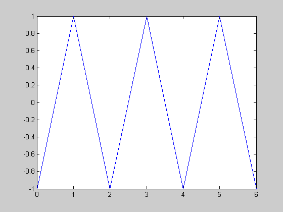
- Let $u(t)$ be the unit step function. Let $f(t)$ be the "triangle
wave" with amplitude 1 and period 2 graphed below.

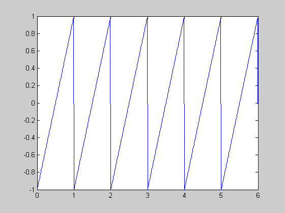
- Let $u(t)$ be the unit step function. Let $f(t)$ be the "sawtooth
wave" with amplitude 1 and period 1 graphed below.

- Sometimes the solution of one constant coefficient linear differential equation will become part of the statement of another such equation. In this case, using Laplace transforms and leaving everything in the frequency domain until the very end is often easiest. Solve the following for $y$ (you don't need to give $x$). $$ \begin{align} \frac{dx}{dt}+4x&=\exp(t), \qquad &x(0)=0 \\ \frac{dy}{dt}+2y&=x(t), \qquad &y(0)=0 \end{align} $$
- Sometimes the solution of one constant coefficient linear differential equation will become part of the statement of another such equation. In this case, using Laplace transforms and leaving everything in the frequency domain until the very end is often easiest. Solve the following for $y$ (you don't need to give $x$). $$ \begin{align} \frac{dx}{dt}+x&=\delta(t), \qquad &x(0)=0 \\ \frac{d^2y}{dt^2}+4y&=x(t), \qquad &y(0)=0,\quad y'(0)=0 \end{align} $$
- Sometimes the solution of one constant coefficient linear differential equation will become part of the statement of another such equation. In this case, using Laplace transforms and leaving everything in the frequency domain until the very end is often easiest. Solve the following for $y$ (you don't need to give $x$). $$ \begin{align} \frac{d^2x}{dt^2}+9x&=3\delta(t), \qquad &x(0)=0,\quad x'(0)=0 \\ \frac{d^2y}{dt^2}+y&=x(t), \qquad &y(0)=0,\quad y'(0)=0 \end{align} $$
- Sometimes the solution of one constant coefficient linear differential equation will become part of the statement of another such equation. In this case, using Laplace transforms and leaving everything in the frequency domain until the very end is often easiest. Solve the following for $y$ (you don't need to give $x$). $$ \begin{align} \frac{d^2x}{dt^2}+9x&=\sin(t), \qquad &x(0)=0,\quad x'(0)=0 \\ \frac{d^2y}{dt^2}+3\frac{dy}{dt}+2y&=x(t), \qquad &y(0)=0,\quad y'(0)=0 \end{align} $$
- Let $f(t)$ be an "impulse train," $$f(t)=\delta(t)+\delta(t-\pi)+\delta(t-2\pi)+\cdots$$ Show the Laplace transform of the solution to $$\frac{d^2x}{dt^2}+4x=f(t),\qquad x(0)=0,\quad x'(0)=0 $$ has a double pole on the imaginary axis, which suggests (but doesn't prove) that this solution might be in resonance. Explain why resonance is reasonable here.
- Let $g(t)$ be the square wave $$g(t) = -1+2\sum_{n=0}^{\infty}(-1)^nu(t-n)$$ Show the Laplace transform of the solution to $$\frac{d^2x}{dt^2}+\pi^2x=g(t),\qquad x(0)=0,\quad x'(0)=0 $$ has a double pole on the imaginary axis, which suggests (but doesn't prove) that this solution might be in resonance. Explain why resonance is reasonable here.
- Solve as a convolution integral. $$\frac{d^2x}{dt^2}-x=e^{-t^2},\qquad x(0)=0,\quad x'(0)=0. $$
- Solve using variation of parameters. $$\frac{d^2x}{dt^2}-x=e^{-t^2},\qquad x(0)=0,\quad x'(0)=0. $$
- Solve using variation of parameters. $$\frac{d^2x}{dt^2}+x=\sec(t),\qquad x(0)=0,\quad x'(0)=0. $$
- Solve as a convolution integral. $$\frac{d^2x}{dt^2}+x=\sec(t),\qquad x(0)=0,\quad x'(0)=0. $$
- The homogeneous solutions to the following equation are $y=x^2$ and $y=x^3$. Solve the initial value problems using variation of parameters, and explain why Laplace transform techniques are not helpful here. $$ x^2\frac{d^2y}{dx^2}-4x\frac{dy}{dx}+6y=3x^5,\qquad y(1)=0,\quad y'(1)=0. $$
- The homogeneous solution to the following equation are $y=x$ and $y=\exp(x).$ Solve the initial value problem using variation of parameters, and explain why Laplace transform techniques are not helpful here. $$ (3x-3)\frac{d^2y}{dx^2}-3x\frac{dy}{dx}+3y=\exp(2x),\qquad y(0)=0,\quad y'(0)=0. $$
- In some situations you may expect a system to experience several shocks in sequence of different amplitudes (think of an earthquake and aftershocks). Solve the initial value problem $$ \frac{d^2x}{dt^2}+2\frac{dx}{dt}+10x=\delta(t)+\frac12\delta(t-1), \qquad x(0)=0,\quad x'(0)=0. $$
- In some situations you may expect a system to experience several shocks in sequence of different amplitudes (think of an earthquake and aftershocks). Solve the initial value problem $$ \frac{d^2x}{dt^2}+2\frac{dx}{dt}+2x= \delta(t)+\frac12\delta(t-2\pi)+\frac12\delta(t-4\pi), \qquad x(0)=0,\quad x'(0)=0. $$
- Graph the solution of the initial value problem $$ \frac{d^2x}{dt^2}+4\pi^2x=\delta(t)-\delta(t-1), \qquad x(0)=0,\quad x'(0)=0. $$ Give a physical explanation for what this problem might represent.
- Solve the linear system $$ \begin{align} \frac{dx}{dt}&=3x-2y+\delta(t),\qquad &x(0)=0 \\ \frac{dy}{dt}&=5x+y,\qquad &y(0)=0 \end{align} $$
- Solve the linear system $$ \begin{align} \frac{dx}{dt}&=3x-2y,\qquad &x(0)=0 \\ \frac{dy}{dt}&=5x+y+\delta(t),\qquad &y(0)=0 \end{align} $$
- Solve the linear system $$ \begin{align} \frac{d^2x}{dt^2}&=5x+2y,\qquad &x(0)=1,\quad x'(0)=0 \\ \frac{d^2y}{dt^2}&=2x+8y,\qquad &y(0)=2,\quad y'(0)=0 \end{align} $$
- Solve the linear system $$ \begin{align} \frac{d^2x}{dt^2}&=2x+6y,\qquad &x(0)=3,\quad x'(0)=0 \\ \frac{d^2y}{dt^2}&=x+y,\qquad &y(0)=1,\quad y'(0)=0 \end{align} $$
- Find and classify the equilibria for $$ \begin{align} \frac{dx}{dt}&=x^2+y^2-2 \\ \frac{dy}{dt}&=x-y \end{align} $$
- Find and classify the equilibria for $$ \begin{align} \frac{dx}{dt}&=x^2+y^2-2 \\ \frac{dy}{dt}&=y-x \end{align} $$
- Find and classify the equilibria for $$ \begin{align} \frac{dx}{dt}&=x^2+y^2-5 \\ \frac{dy}{dt}&=xy-2 \end{align} $$
- Find and classify the equilibria for $$ \begin{align} \frac{dx}{dt}&=5-x^2-y^2 \\ \frac{dy}{dt}&=xy-2 \end{align} $$
- Find and classify the equilibria for $$ \begin{align} \frac{dx}{dt}&=y-x^2 \\ \frac{dy}{dt}&=x-y^2 \end{align} $$
- Find and classify the equilibria for $$ \begin{align} \frac{dx}{dt}&=x^2-y^2 \\ \frac{dy}{dt}&=x-2y+2 \end{align} $$
- In the paradigm we considered the problem $$ \begin{align} \frac{dx}{dt}&=4x-2xy \\ \frac{dy}{dt}&=xy-3y \end{align} $$ This is an example of a "predator-prey" population model. $x$ represents the population of a prey species that naturally grows exponentially but is controlled by predation by the predator species (hence the $-2xy$ term). $y$ represents the population of a predator species that needs to find sufficient prey to survive (hence the $+xy$ term). As observed in the text, this system has an equilibrium point at $(3,2)$, but linearization failed to classify it. However, using the fact that $\displaystyle \frac{dy}{dx} = \frac{dy/dt}{dx/dt}$ we can rewrite this system as a first-order equation in $x$ and $y$. Solve this equation. Note that this tells you how $x$ and $y$ are related, but doesn't tell you how they evolve with respect to $t$.
- Now that you've found the"solution" (relating $x$ and $y$ to each other but not to $t$) for $$ \begin{align} \frac{dx}{dt}&=4x-2xy \\ \frac{dy}{dt}&=xy-3y \end{align} $$ in the previous problem, find the implicit formula for $y$ and $x$ for the initial value problem with $x(0)=2$, $y(0)=1/2$. Sketch the graph (wolframalpha.com may be helpful here since your solution will be a messy implicit formula). Put arrows on your sketch showing how the point $(x(t),y(t))$ will move around the "orbit" you've sketched in the $xy-\text{plane}$ as $t$ increases. Mark the equilibrium $(3,2)$ (note that it is not in the center of the orbit). Write a short explanation in paragraph form for what this solution predicts about the behavior of the populations of the prey, $x$, and the predators, $y$.
- The basic "competitive species" model is $$ \begin{align} \frac{dx}{dt}&=ax-mxy \\ \frac{dy}{dt}&=by-nxy \end{align} $$ where $x$ and $y$ represent the populations of two competing species, $a$ and $b$ are the growth rates of each species, and $m$ and $n$ reflect competitive pressures between the species. All coefficients are positive, $a,b,m,n > 0.$ Find the equilibria for this model. Your answers will be expressed in terms of $a$, $b$, $m$, and $n.$
- Classify the equilibria you found for the competitive species model in the previous problem. Note that there is no stable equilibrium for this model.
- Using the fact that $\displaystyle \frac{dy}{dx}=\frac{dy/dt}{dx/dt}$, rewrite the competitive species system as a first order equation in $x$ and $y.$ Solve this equation. Note that this tells you how $x$ and $y$ are related, but doesn't tell you how they evolve with respect to $t.$
- For the competitive species model, graph the curves $dx/dt=0$ and $dy/dt=0.$ Draw arrows to show how the populations are growing or shrinking in the regions defined by those curves and use those arrows to sketch some solution curves in the $xy$-plane. Note that the graphical technique here is significantly easier than trying to plot points using the formula found in the previous problem.
- Ernst Mayr in Populations, Species and Evolution wrote,
"In sum: two species cannot indefinitely coexist in the same locality if they have identical ecological requirements. ... The validity of this exclusion principle has been tested in numerous laboratory experiements in which mixed populations of two species were established in a uniform environment. In virtually every case, one of the two species was eliminated sooner or later."
Write a short explanation of whether this principle is true for the competitive species model we have been considering in the previous problems. - One unrealistic feature of the basic competitive species model considered in the previous problems is that one of the populations will tend to infinity. Create a (slightly) more complicated model for competitive species for which populations undergo logistic growth (rather than exponential growth) in the absence of a competitor.
| f(t) |
$\qquad\qquad\qquad$ | F(s) |
|||
|---|---|---|---|---|---|
| 1. | $\cosh(bt)$ | $\displaystyle\frac{s}{s^2-b^2}$ | |||
| 2. | $\sinh(bt)$ | $\displaystyle\frac{b}{s^2-b^2}$ | |||
| 3. | $e^{at}\cosh(bt)$ | $\displaystyle\frac{s-a}{(s-a)^2-b^2}$ | |||
| 4. | $e^{at}\sinh(bt)$ | $\displaystyle\frac{b}{(s-a)^2-b^2}$ |
If you have any problems with this page, please contact bennett@math.ksu.edu.
©2010, 2014 Andrew G. Bennett