Launch the Complex Function Grapher

Introduction

In class we discussed connections between exp(z), sin(z), and cos(z) that could be deduced from their Taylor series. This week we will use the connections between complex exponentials and pairs of sines and cosines to find real solutions to linear constant coefficient differential equations. In this studio we will look at the connections between these geometrically. We will also look at some other ideas about complex functions and their graphs, which will be helpful in some future courses (particularly if you study control theory).

Assignment

1. Graph exp(pi z). According to Euler's formula, we should expect exp(pi z) = cos(pi z/i) + i sin(pi z/i) to be periodic, since cos(z) and sin(z) are periodic. How does the periodicity show up in the graph? What is the period of exp(pi z)?

---

The hyperbolic cosine and hyperbolic sine are defined as cosh(z) = (exp(z)+exp(-z))/2 and sinh(z) = (exp(z)-exp(-z))/2. When these functions are introduced in calculus 2, it is often unclear why they are called a sine and cosine. The next two problems address this issue.

---

2. Graph cos(pi z) and cosh(pi z). How are the two graphs related?

3. Graph i*sin(pi z) and sinh(pi z). How are the two graphs related? What is the relationship between i*sin(pi z) and sinh(pi z)?

---

In the ordinary two-dimensional graph of y² = x, we don't have y as a function of x since the graph fails the vertical line test, that is a given value of x, say x = 4, will give rise to two different values of y, both y = 2 and y = -2. 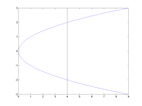We deal with this by defining the square root function to always give the positive square root. We can also speak of the two branches of the square root function, the positive square root and the negative square root, which together make up the graph of y² = x. Of course, as a real-valued function, the square root function is only defined for x >= 0. But the point of complex numbers is that you can now take square roots of negative numbers, indeed of any number. In the next two problems we'll try to develop a sense of the two branches of sqrt(z) for the complex plane.

---

4. Graph sqrt(z) and -sqrt(z). Observe the "branch cut" along the negative real axis. Explain why can't we define a branch of square root which is continuous over the whole plane? Hint: The complex numbers e^iθ trace out a circle around the origin of radius 1 starting and ending at -1 as θ varies from -π to π. What are the values of sqrt(e^iθ) at the beginning and end of the circle?

5. We could build a single graph of the real variables y² = x by stitching the two branches of the square root functions together. How could you stitch the two branches of the square root functions together to get a single graph for the complex case? Hint: The stitching will give you a figure that would have to intersect itself in three dimensions, but since complex graphs are actually 4 dimensional there is the extra room needed to stitch things together.

---

The last topic we will consider are some tricks for finding zeros and poles of complex functions. These tricks can later be used to recognize whether certain systems are stable or unstable. They can also lead to a proof of the fundamental theorem of algebra (this is a math class - you should expect us to talk some about theorems and proofs :)

---

Look at the following functions in the complex function grapher. The Top View will be most useful, but looking at a couple of the examples that have poles using the Side View will help you understand why we use the word "poles" for these points.

• f(z) = z
• f(z) = z^2
• f(z) = z^2+1
• f(z) = 1/z
• f(z) = 1/z^2
• f(z) = (z^2 + 1)/z
6. How can you recognize the zeros and poles of the functions from just looking at the colors you see in the Top View?

7. How can you distinguish a single root from a double root or a single pole from a double pole?

8. How can you distinguish the zeros from the poles by looking at the colors you see in the Top View?

Once you learn to recognize zeros and poles, you can look for patterns in how the colors work.

9. Fill in the following table. Count roots and poles of the following functions with multiplicity (i.e. a double root counts as two). Also count how many times you cycle through the rainbow as you move around the edge of the graph window. When counting the rainbows around the edge of the graph, count rainbows that move counterclockwise as you go from red to yellow to green to blue to violet as positive and rainbows that go clockwise as negative.

   Function	# Roots	# Poles	Rainbows at the edge
   (z+1)(z-1)^2
   (z^2+z)/(z-1)
   (z^2-2)z^2/(z^2+1)

10. Look at the values you found in the table above. Can you find a pattern for the rainbows around the edge in terms of the # of roots and the # of poles? This pattern is called the principle of the argument

Now from the principle of the argument, that means the (# roots) - (# poles) of the polynomial is n. But a polynomial has no poles (since it has no denominator), so the polynomial must have exactly n roots (including complex roots and counting multiplicity). And this is exactly the Fundamental Theorem of Algebra. In Math 630, you can learn how to prove these patterns must always hold, but just by experimentation I hope you can see these patterns hold, and then understand why these patterns imply the Fundamental Theorem of Algebra is true. In the next chapter we will discover that knowing where the poles of the "Laplace transform" of the solution of a differential equation tells us a great deal about the stability of the system being modeled, and techniques like this can help us determine where poles are located in the complex plane.