Applications
Mechanical Vibrations
Consider a mass on a spring. The forces acting on the mass are gravity with a force $mg$, where $m$ is the mass and $g$ is the acceleration of gravity $(9.8\text{m}/sec^2)$, the restoring force of the spring with a force $-kl$, where $k$ is the spring constant, $l$ is how much the spring is stretched and the negative sign denotes the force is pulling toward $l=0$, and the damping of the spring (friction) acting with a force $-cv$, where $c$ is the damping constant, $v$ is the velocity and the negative sign denotes that the force acts in opposition to the motion. Now we choose our coordinates for the problem to have $x=0$ at the equilibrium length of the spring $s$, where $mg=ks$. Note that with this choice, $l=x+s$. We also choose $x>0$ to be when the spring is stretched farther down from equilibrium (this is why we use $mg$ for gravity and not $-mg$). So the total force on the spring is $$ \begin{align} mg - kl - cv &= mg - k(s+x) - cv \\ &= mg - ks - kx - cv \\ &= -kx -cv \end{align} $$ But by Newton's second law of motion, $\text{force} = ma $ where $m$ is mass and $a$ is acceleration. So $$ ma = -kx - cv $$ Now if we remember that velocity is the derivative of position with respect to time and acceleration is the second derivative of position with respect to time, we have our final equation for "free" motion of a spring-mass system $$ m\frac{d^2x}{dt^2}+c\frac{dx}{dt}+kx=0 $$ where $m$ is mass, $c$ is the damping constant, $k$ is the spring constant, $x$ is position and $t$ is time. This basic setup will be useful for most mechanical vibration problems, but typically with an additional term. The equation for "free" motion above assumed that the only force acting on the mass was gravity and we could choose coordinates to allow us to ignore that force. However, in many situations there may be an external force $F(t)$ involved which we can't (and wouldn't want to) ignore. For example, a running motor will cause vibrations in attached parts. This leads to the equation for "forced" motion of a spring-mass system $$ m\frac{d^2x}{dt^2} + c\frac{dx}{dt} + kx = F(t)$$ where $F(t)$ is the external force. In this chapter we will mainly consider periodic external forces of the form $F(t)=A\cos(\omega t)$, which are very common in practice.LRC Circuits
Electric circuits are analyzed using exactly the same equations as spring-mass systems. We look at the current $I$ flowing through the circuit, where $\displaystyle I=\frac{dQ}{dt}$ where $Q$ is charge. $Q$ is measured in coulombs while $I$ is measured in amperes, which are coulombs/second. The "electromotive force" $E$ powering the circuit is measured in volts (note that pressure may be a better metaphor). An LRC circuit with an AC power source includes the
following components. As current flows through the loops of a coil,
the spinning current induces a magnetic field. If the current flow
changes, then the magnetic field changes. A changing magnetic field inside
the loops will then induce a current. This acts like mass in a spring-mass
system, since the induced current opposes the change in the current, just
as mass measures opposition to change in momentum. A coil has "inductance"
$L$, which is measured in henrys. Voltage drop across a coil is given by
$\displaystyle V=L\frac{dI}{dt}=L\frac{d^2Q}{dt^2}$.
A resistor does what it sounds like, it resists the flow of
current. Resistance $R$, measured in ohms, plays the role of friction. The
voltage drop across a resistor is $\displaystyle V=RI=R\frac{dQ}{dt}$.
A capacitor stores charge on parallel plates separated by a
dielectric.
The amount of charge is proportional to the impressed voltage, $Q=CV$, or
$\displaystyle V=\frac{1}{C}Q$. Capacitance $C$ is measured in farads,
which are coulombs per volt. Since the
charge will be released as the voltage drops, the capacitor plays the role
of the spring, storing energy and then releasing it later. In fact, $1/C$
is called the "elastance" of the circuit and plays the role of the spring
constant (and has units of "daraf", though reciprocal farad is
the more boring preferred term).
Finally, the AC power source produces an alternating voltage described by
a sinusoidal function, $E(t)=V_0\cos(\omega t)$. $V_0$ is the peak
amplitude and $\omega$ is the circular frequency. Note that when voltages
are given, you typically use the root-mean-square amplitude rather than
the peak amplitude, so a 120 volt supply would correspond to a peak
amplitude of $120\sqrt2\approx 170$ volts. Similarly, frequency is
usually given in Hertz, which are cycles per second, while circular
frequency is measured in radians per second, so a 60 Hertz supply has
$\omega=60\times2\pi=120pi$ since 2π radians equals one full cycle.
An LRC circuit with an AC power source includes the
following components. As current flows through the loops of a coil,
the spinning current induces a magnetic field. If the current flow
changes, then the magnetic field changes. A changing magnetic field inside
the loops will then induce a current. This acts like mass in a spring-mass
system, since the induced current opposes the change in the current, just
as mass measures opposition to change in momentum. A coil has "inductance"
$L$, which is measured in henrys. Voltage drop across a coil is given by
$\displaystyle V=L\frac{dI}{dt}=L\frac{d^2Q}{dt^2}$.
A resistor does what it sounds like, it resists the flow of
current. Resistance $R$, measured in ohms, plays the role of friction. The
voltage drop across a resistor is $\displaystyle V=RI=R\frac{dQ}{dt}$.
A capacitor stores charge on parallel plates separated by a
dielectric.
The amount of charge is proportional to the impressed voltage, $Q=CV$, or
$\displaystyle V=\frac{1}{C}Q$. Capacitance $C$ is measured in farads,
which are coulombs per volt. Since the
charge will be released as the voltage drops, the capacitor plays the role
of the spring, storing energy and then releasing it later. In fact, $1/C$
is called the "elastance" of the circuit and plays the role of the spring
constant (and has units of "daraf", though reciprocal farad is
the more boring preferred term).
Finally, the AC power source produces an alternating voltage described by
a sinusoidal function, $E(t)=V_0\cos(\omega t)$. $V_0$ is the peak
amplitude and $\omega$ is the circular frequency. Note that when voltages
are given, you typically use the root-mean-square amplitude rather than
the peak amplitude, so a 120 volt supply would correspond to a peak
amplitude of $120\sqrt2\approx 170$ volts. Similarly, frequency is
usually given in Hertz, which are cycles per second, while circular
frequency is measured in radians per second, so a 60 Hertz supply has
$\omega=60\times2\pi=120pi$ since 2π radians equals one full cycle.
Examples of Free Motion
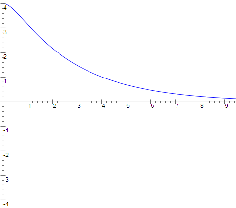
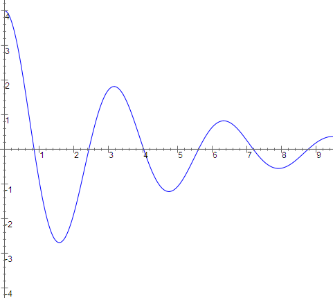
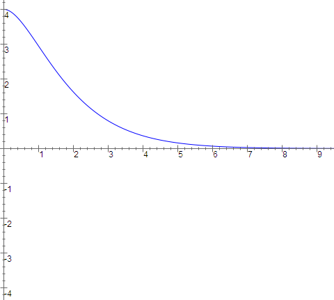
We now solve the free motion equation in general and see what we can deduce about the behavior of such a system. First we assume there is no damping $(c=0)$. Then the general solution is $$ \begin{align} x(t) &= a \cos(\omega t) + b \sin(\omega t) \\ &= A \cos(\omega(t+\phi)) \end{align} $$ depending on which way you want to write the formula. Here $\omega$ is $\sqrt{k/m}$. This is simple harmonic motion with amplitude $A$, circular frequency $\omega$ and phase shift $\phi$.
Examples of Forced Motion
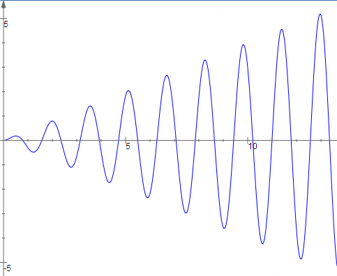
We start with the undamped case $(c=0)$. We have solved the homogeneous problem in the previous section, obtaining $A\cos(\omega_0(t + \phi))$ where $\omega_0 =\sqrt{k/m}$ is called the natural frequency of the spring-mass system. We will now consider the particular solution of $$m\frac{d^2x}{dt^2}+kx=F_0\cos(\omega t)$$ Since $F_0 \cos(\omega t) = \Re[F_0 e^{i\omega t}]$, we will try to find the particular solution for the complex problem and then take the real part. So we guess $$ \begin{align} z&=ae^{i\omega t} \\ z'&=i\omega ae^{i\omega t} \\ z''&=-\omega^2ae^{i\omega t} \end{align} $$ So we get $$ \begin{align} -m\omega^2ae^{i\omega t}+kae^{i\omega t}&=F_0e^{i\omega t} \\ a&=\frac{F_0}{-m\omega^2+k}=\frac{F_0}{m(\omega_0^2-\omega^2)} \end{align} $$ and taking the real part of $ae^{i\omega t}$ yields a particular solution of $$ x(t)=\frac{F_0}{m(\omega_0^2-\omega^2)}\cos(\omega t)$$ Note that the particular solution has the same frequency as the forcing function but that the amplitude is divided by a factor $m(\omega_0^2 - \omega^2)$. We would expect to see that mass would be inversely proportional to the displacement generated by a fixed force, but it may be something of a surprise that the frequency plays such a large role. The underlying physical intuition is that the spring wants to oscillate at its natural frequency, and the closer the forcing function is to the natural frequency, the more the forcing function and the spring will work together and not in opposition, hence the larger amplitude of the response. The general solution is then $$x(t)=\frac{F_0}{m(\omega_0^2-\omega^2)}\cos(\omega t)+A\cos(\omega_0(t+\phi))$$ If we plot out the solution curves, we will see the phenomenon of beats arising. This is most easily seen if $\omega$ and $\omega_0$ are close. Then the amplitude of the solution will steadily increase as the forcing function pours ever greater amounts of energy into the system. However, if the forcing function is not exactly in sync with the natural frequency of the system (that is $\omega\ne\omega_0$) then eventually the forcing function will become out of phase with the natural frequency. Then the force applied to the system will reduce the amplitude and the "beat" will die off. At the end of the beat, the forcing function will have worked its way back in sync with the natural frequency and the pattern will start all over again.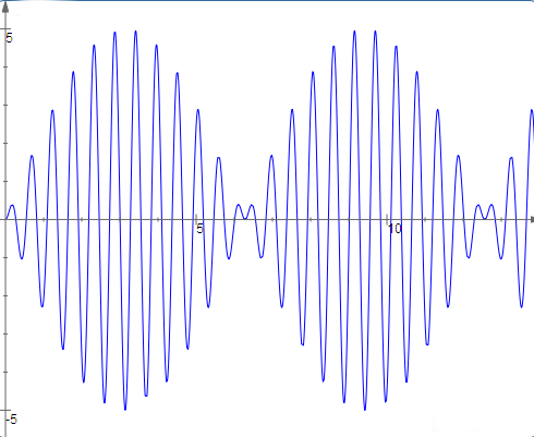
If you have any problems with this page, please contact bennett@ksu.edu.
©1994-2025 Andrew G. Bennett